

 SYLLABUS Previous: 3.3 Improved model using
Up: 3.3 Improved model using
Next: 3.3.2 Itô lemma
SYLLABUS Previous: 3.3 Improved model using
Up: 3.3 Improved model using
Next: 3.3.2 Itô lemma
3.3.1 Wiener process and martingales

[ SLIDE
SDE -
Wiener -
Markov ||
VIDEO
modem -
LAN -
DSL]
Although it is not possible to predict with any certainty the spot price
 of an asset in an efficient market,
sect.2.1.1 demonstrated in that
possible realizations can be simulated with
their probability of occurrence by summing price increments
of an asset in an efficient market,
sect.2.1.1 demonstrated in that
possible realizations can be simulated with
their probability of occurrence by summing price increments  over
small steps in time
over
small steps in time  .
Separating the
deterministic
.
Separating the
deterministic  from the
remaining random component
from the
remaining random component
 ,
the evolution of the random variable
satisfies a
stochastic differential equation
,
the evolution of the random variable
satisfies a
stochastic differential equation
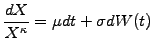 |
(3.3.1#eq.1) |
where  =0 (alt. 1) chooses between the normal (alt. log-normal)
distribution of increments discussed previously in (2.1.1#eq.1).
Integrating over time, the first term yields a uniform (alt.
exponential) growth with a rate
=0 (alt. 1) chooses between the normal (alt. log-normal)
distribution of increments discussed previously in (2.1.1#eq.1).
Integrating over time, the first term yields a uniform (alt.
exponential) growth with a rate  that accounts for example for
a continuous payment of a fixed dividend (alt. a compounded interest
rate).
The second term reproduces a random walk proportional to the market
volatility
that accounts for example for
a continuous payment of a fixed dividend (alt. a compounded interest
rate).
The second term reproduces a random walk proportional to the market
volatility  , using a so-called
Wiener process
that has the following properties
, using a so-called
Wiener process
that has the following properties
- The Wiener increment
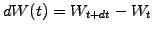 over a time step
is a random variable drawn from a normal distribution with zero
mean and a time-step variance
over a time step
is a random variable drawn from a normal distribution with zero
mean and a time-step variance
![$ \mathcal{N}[0,dt]$](s3img78.gif) (1.4#eq.5).
Extensions to other distributions (e.g. 2.1.1#eq.3) are possible.
(1.4#eq.5).
Extensions to other distributions (e.g. 2.1.1#eq.3) are possible.
- The Wiener increment is independent of the past. Using the
definition (1.4#eq.3) for the correlation, this is satisfied
when
![$ E[dW(t_1)dW(t_2)]=0, \forall t_1<t_2$](s3img79.gif) .
.
A convenient way of writing this is
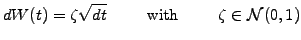 |
(3.3.1#eq.2) |
where different realizations of the random variable  are
generated using random numbers
are
generated using random numbers  that are normally distributed.
This construction provides the mathematical foundation for the
Monte-Carlo simulations, where the
mean value of the increment
that are normally distributed.
This construction provides the mathematical foundation for the
Monte-Carlo simulations, where the
mean value of the increment
![$\displaystyle E[dX] = E[X^\kappa (\mu dt +\sigma dW(t))] = \mu X^\kappa dt$](s3img83.gif) |
(3.3.1#eq.3) |
and the variance
![$\displaystyle \mathrm{Var}[dX] = E[dX^2] - E[dX]^2 = E[(X^\kappa \sigma dW(t))^2] = \sigma^2 X^{2\kappa} dt$](s3img84.gif) |
(3.3.1#eq.4) |
are matched with historical data to forecast possible evolutions into
the future. Third or even higher order moments of the probability
distribution can in principle also be matched; experience, however,
shows that little is to be gained from such a procedure.
A better description of the market is obtained by performing a
principal components analysis
[19], where several imperfectly correlated random variables
are identified and then superposed to drive increments of the form
![$\displaystyle dX=\sum_i X_i^\kappa [\mu_i dt +\sigma_i dW_i(t)]$](s3img85.gif) |
(3.3.1#eq.5) |
where
![$ \rho_{ij} \in [-1;1]$](s3img90.gif) is a correlation factor.
The first component typically accounts for 80-90% (and the first three
for up to 95-99%) of the variance observed in the market price of forward
rates [19].
is a correlation factor.
The first component typically accounts for 80-90% (and the first three
for up to 95-99%) of the variance observed in the market price of forward
rates [19].
Note that the forecast value for the price of a share  or an
interest rate
or an
interest rate  constructed using Wiener increments depends
only the present value: this independence from the past is known in
mathematics as the Markov property.
Also note that a suitable choice of a
numeraire can always be found to normalize
random variables and make them risk-neutral by scaling out the drift observed
in the real world: called martingales,
such variables play an important role in the construction of financial models.
constructed using Wiener increments depends
only the present value: this independence from the past is known in
mathematics as the Markov property.
Also note that a suitable choice of a
numeraire can always be found to normalize
random variables and make them risk-neutral by scaling out the drift observed
in the real world: called martingales,
such variables play an important role in the construction of financial models.
SYLLABUS Previous: 3.3 Improved model using
Up: 3.3 Improved model using
Next: 3.3.2 Itô lemma