

 SYLLABUS Previous: 3.1 Option pricing for
Up: 3 FORECASTING WITH UNCERTAINTY
Next: 3.3 Improved model using
SYLLABUS Previous: 3.1 Option pricing for
Up: 3 FORECASTING WITH UNCERTAINTY
Next: 3.3 Improved model using
3.2 Simple valuation model using binomial trees

[ SLIDE
tree -
delta hedging -
transition probability -
matching volatility -
recipe ||
VIDEO
modem -
LAN -
DSL ]
A single step binomial forecast provides only a crude approximation for
the fair price of an option before it expires.
To increase the accuracy of the model, an obvious improvement would be to
extend the number of possible outcomes; the evolution of the forecast price
could also be modeled more accurately by allowing them to reverse trends
during the calculation.
Both can be achieved by dividing the lifetime of the option [0;T]
into a number smaller time intervals of duration Dt
and performing the calculation recursively with the binomial tree
model sketched in (3.2#fig.1).
In addition, we show here how a tree is constructed to reproduce log-normal
price increments that are typical for stock: rather than adding / subtracting
a constant as in the previous sect.3.1 (for a normal distribution),
possible realizations are here obtained by multiplying / dividing by a
constant factor (for a log-normal distribution).
Figure 3.2#fig.1:
Sketch showing how a sequence of two binomial steps in a tree that can
be used to simulate possible realizations of a stockmarket price with
 .
The time step
.
The time step
 has been adjusted so that two levels
span the entire lifetime of the option
has been adjusted so that two levels
span the entire lifetime of the option  .
More levels yield a more accurate result.
.
More levels yield a more accurate result.
|
|
For each step starting with the present value of the underlying S0 two new forcasts are obtained by multiplying the value on each node by
the factors u or d to mimic possible movements up or down until the entire lifetime of the
option is covered by the tree.
A perfectly hedged portfolio is then constructed starting from every
branching point closest to the expiry date (work backwards from the
right of (3.2#fig.1), by combining an amount delta of the underlying
with a (conventionally short) position of a (positively correlated)
option. By demanding that the portfolio be risk free, the movement up
or down produce the same return and a new value is obtained for delta
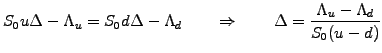 |
(3.2#eq.1) |
Since a perfectly hedged portfolio carries no risk at all, the standard
no-arbitrage argument shows that it can
be discounted back one step in time using the risk free interest rate r This discounted value (3.2#eq.2, left hand side) has to be
equal to the cost of setting up the portfolio before the step is taken
(right hand side):
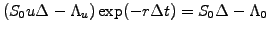 |
(3.2#eq.2) |
Substituting the hedging factor delta (3.2#eq.1) and
rearranging the terms, this yields an expression to calculate
the fair value of an option one step back at a time
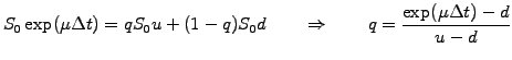
![$\displaystyle \Lambda_0 = [p\Lambda_u +(1-p)\Lambda_d]\exp(-r\Delta t) \qquad\mathrm{with}\qquad p=\frac{\exp(r\Delta t)-d}{u-d}$](s3img61.gif) |
(3.2#eq.3) |
The parameter p can be interpreted as the probability of the forecast price moving up and (1-p) the probability that it will move down in the tree. The scaling factors (u,d) control the amplitude of the change and have to be carefully chosen
 |
(3.2#eq.4) |
to reproduce the drift and the volatility observed in the real markets
(quants read below).
Although the importance will only appear later, simply note here that
the expected value of the underlying calculated using the probability
(3.2#eq.3)
![$\displaystyle E[S]=pS_0u -(1-p)S_0d = p(u-d)S_0 +S_0s = S_0\exp(r\Delta t)$](s3img63.gif) |
(3.2#eq.5) |
grows, on average, exactly at the risk free interest rate.
Using the probability (3.2#eq.3) therefore implies that the return
on the underlying stock is equal to the risk free rate m=r.
Quants: matching the parameters (u,d) with drift and volatility.
For clarity, distinguish the probability of a price moving up in the tree p from the probability of the price moving up in the real world q. In the presence of drift, the real world price of the underlying grows
exponentially (3.2#eq.6, left hand side), which should be
reproduced by the expectation E[S] from the price forecast in the tree (right hand side):
 |
(3.2#eq.6) |
In the same manner, the real world variance (square of volatility, left)
has to be matched with the variance Var[S]=E[S2]-E[S]2 from the price forecast in the tree (right):
![$\displaystyle \sigma^2\Delta t = qu^2 +(1-q)d^2 -[qu +(1-q)d]^2$](s3img65.gif) |
(3.2#eq.7) |
Substitute the real world probability (3.2#eq.6) into
(3.2#eq.7)
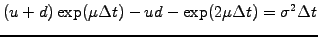 |
(3.2#eq.8) |
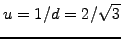
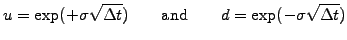
and expand to first order in the small time steps by writing exp(mD)~ 1 +mD. The symmetric solution u=1/d is generally chosen and is the one given in (3.2#eq.4).
To summarize, calculations using binomial trees for the stockmarket can be
organized as follows
- Divide the entire lifetime of the option into a finite number of
steps N, ranging from only a few (by hand) up to 30 (using a computer
to evaluate 31 possible outcomes that are connected with 230~ 1 billion possible paths).
- Forecast the underlying forward in time (trunk
 leaves),
choosing (u,d) according to (3.2#eq.4) to reproduce the historical
volatility observed in a real market.
leaves),
choosing (u,d) according to (3.2#eq.4) to reproduce the historical
volatility observed in a real market.
- Work backward in time (trunk
 leaves) starting from the
terminal option payoff; for every neighboring branching point, calculate
the hedging delta (3.2#eq.1) and the option price at the
previous time step (3.2#eq.3).
In the case of American options, substitute the (larger)
intrinsic value
that can be obtained from an early exercise when the calculated price
drops below this intrinsic value.
leaves) starting from the
terminal option payoff; for every neighboring branching point, calculate
the hedging delta (3.2#eq.1) and the option price at the
previous time step (3.2#eq.3).
In the case of American options, substitute the (larger)
intrinsic value
that can be obtained from an early exercise when the calculated price
drops below this intrinsic value.
- The final result is obtained on the trunk of the tree and is an
approximation of the fair value of the option before the expiry date,
with an accuracy proportional to 230.
Because it involves only simple mathematics, binomial trees are ideally
suited to develop an intuition for option pricing (exercise 3.01, 3.02).
Some practitioners even use trees to evaluate option prices with a computer:
the forthcoming sections will show that differential calculus provides a far
better framework to account for the features appearing in exotic contracts.
Indeed, without having to account for these features, the computer is not
really needed: the price can simply be calculated from an analytic solution
of the Black-Scholes differential equation, which we are about to derive.
SYLLABUS Previous: 3.1 Option pricing for
Up: 3 FORECASTING WITH UNCERTAINTY
Next: 3.3 Improved model using
![\includegraphics[width=6cm]{figs/tree2.eps}](s3img58.gif)