

 SYLLABUS Previous: 6.2.1 The Black-Scholes equation
Up: 6.2 Methods for American
Next: 6.3 Computer quiz
SYLLABUS Previous: 6.2.1 The Black-Scholes equation
Up: 6.2 Methods for American
Next: 6.3 Computer quiz
                                                       //--- CONSTRUCT MATRICES
      BandMatrix a = new BandMatrix(3, f.length);      // Linear problem
      BandMatrix b = new BandMatrix(3, f.length);      //  a*fp=b*f=c
      double[]   c = new double[f.length];
      double htm = dxk*(1-tune)/4;                     // Quadrature coeff
      double htp = dxk*(1+tune)/4;
      double halpha = dtau/dxk;                        // PDE coefficient
      for (int i=0; i<=n; i++) {
        a.setL(i,   htm -halpha* theta    );
        a.setD(i,2*(htp +halpha* theta   ));
        a.setR(i,   htm -halpha* theta    );
        b.setL(i,   htm -halpha*(theta-1) );
        b.setD(i,2*(htp +halpha*(theta-1)));
        b.setR(i,   htm -halpha*(theta-1) );
      }
      c=b.dot(fm);
      a.setL(0,0.);a.setD(0,1.);a.setR(0,0.);c[0]=0;   // First equation idle

                                                       //--- BC + SOLVE
      if (scheme.equals(vmarket.EUNORM)) {             // European option
        a.setL(1, 0.);a.setD(1,1.);a.setR(1,0.);       //   in-money: Dirichlet
        c[1]=Math.exp(0.5*k2m1*xk0+0.25*k2m1*k2m1*tau);
        a.setL(n,-1.);a.setD(n,1.);a.setR(n,0.);c[n]=0.; // out-money: Neuman
        f=a.ssor3(c,fm);                               // conventional-SSOR
        y0=strike*Math.exp(-rate*time);

      } else if (scheme.equals(vmarket.AMNORM)) {      // American option
        double[] min = new double[f.length];           // Obstacle
        double[] max = new double[f.length];
        for (int i=0; i<=n; i++) {
          xk=xk0+(i-1)*dxk;
          min[i]=Math.exp((0.25*k2m1*k2m1 +k1)*tau) *
                 Math.max(0., Math.exp(0.5*k2m1*xk) -
                              Math.exp(0.5*k2p1*xk)  );
          max[i]=Double.POSITIVE_INFINITY;
          fm[i]=Math.max(min[i],f[i]);                 //   IC interp error
        }
        a.setL(1, 0.);a.setD(1,1.);a.setR(1,0.);       // In-money: Dirichlet
        c[1]=Math.max(min[1],Math.exp(0.5*k2m1*xk0+0.25*k2m1*k2m1*tau));
        a.setL(n,-1.);a.setD(n,1.);a.setR(n,0.);c[n]=0.; //out-money: Neuman
        double precision = strike*Math.pow(10.,-6);      // relativ.to strike
        int maxIter = 30;
        double w = 1.2;                                // relaxation parameter
        f=a.ssor3(c,fm,min,max,precision,w,maxIter);   // projected-SSOR
        fp[0]=strike;
      }
The code has intentionally been restricted for the case of American put
options, leaving the complete implementation with call options to the
reader (exercise 6.06). Note that the terminal and boundary conditions
have been specified here in log-normal variables (4.4.2#eq.4),
using the same definitions as for the finite differences in
sect.4.4.2
SYLLABUS Previous: 6.2.1 The Black-Scholes equation Up: 6.2 Methods for American Next: 6.3 Computer quiz
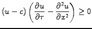
![$\displaystyle \int_{x_-}^{x_+} dx \; \left[ (v-u) \frac{\partial u}{\partial \t...
...\frac{\partial u}{\partial x}\right)\frac{\partial u}{\partial x} \right] \ge 0$](s6img68.gif)
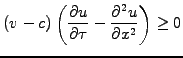
![$\displaystyle \int_{x_-}^{x_+} dx \; \left[ \left(\sum_{i=0}^{n-1} (v_i-u_i) e_...
...rime(x) \right) \left(\sum_{j=0}^{n-1} (u_i e_j^\prime(x) \right) \right] \ge 0$](s6img70.gif)
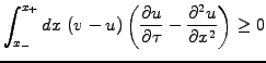
![$\displaystyle \sum_{i=0}^{n-1}\sum_{j=0}^{n-1} (v_i-u_i) \left[ \frac{\partial u_j}{\partial \tau} <e_i\vert e_j> +u_i <e_i^\prime\vert e_j^\prime> \right] \ge 0$](s6img71.gif)
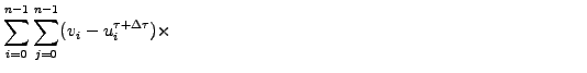
![$\displaystyle \sum_{i=0}^{n-1}\sum_{j=0}^{n-1} (v_i-u_i^{\tau+\Delta\tau}) \lef...
...t e_j^\prime> +\bar{\theta} u_i^\tau <e_i^\prime\vert e_j^\prime> \right] \ge 0$](s6img74.gif)
![$\displaystyle \sum_{j=0}^{n-1}\left(
\left[<e_i\vert e_j> +\Delta\tau\theta<e_i...
... -\Delta\tau\bar{\theta}<e_i^\prime\vert e_j^\prime>\right]
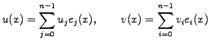
u_j^\tau\right) = 0$](s6img77.gif)