

 SYLLABUS Previous: 4.5.1 Forecast possible realizations
Up: 4.5 Methods for European
Next: 4.6 Computer quiz
SYLLABUS Previous: 4.5.1 Forecast possible realizations
Up: 4.5 Methods for European
Next: 4.6 Computer quiz
4.5.2 Expected value of an option from sampled data

[ SLIDE
open -
scheme -
code || same
VIDEO as previous section:
modem -
LAN -
DSL]
To develop your intuition, let us first define the transition probability
![$ p[S,t;S^\prime,T]$](s4img176.gif) measuring the likelyhood that an asset evolves from
the present value to the terminal value
measuring the likelyhood that an asset evolves from
the present value to the terminal value
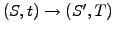 :
weighted by the terminal payoff of an option
:
weighted by the terminal payoff of an option
 , this can
be used to evaluate the expected return from a particular realisation of
the market. Summing the weighted returns from all possible realisations
with the proper Jacobian, the present value of an option could be
calculated from
, this can
be used to evaluate the expected return from a particular realisation of
the market. Summing the weighted returns from all possible realisations
with the proper Jacobian, the present value of an option could be
calculated from
![$\displaystyle V(S,t) = \exp[-r(T-t)]\int_0^\infty p[S,t;S^\prime,T] \Lambda(S^\prime) \frac{dS^\prime}{{S^\prime}^\kappa}$](s4img179.gif) |
(4.5.2#eq.1) |
where the expected terminal payoff has been discounted back to the present
time  by multiplication of the factor
![$ \exp[-r(T-t)]$](s4img180.gif) . This expression
can be identified with the analytical solution (4.3.2#eq.11) and shows
that the price of an option can also be calculated as the present value of
the expected return, using a random walk in a risk-neutral world
where the drift is replaced by the spot rate minus the
dividend yield
. This expression
can be identified with the analytical solution (4.3.2#eq.11) and shows
that the price of an option can also be calculated as the present value of
the expected return, using a random walk in a risk-neutral world
where the drift is replaced by the spot rate minus the
dividend yield  .
(Note the analogy with the delta hedging, where the risk has been
eliminated to obtain a Black-Scholes equation that is also independent
of the drift
.
(Note the analogy with the delta hedging, where the risk has been
eliminated to obtain a Black-Scholes equation that is also independent
of the drift  .)
.)
Instead of calculating a complicated n-dimensional path-dependent integral
with transition probabilities
![$ p[S_i,t_i;S_j,t_j\vert\mathcal{C}_j]$](s4img183.gif) that are
subject to multiple conditions
that are
subject to multiple conditions

![\begin{displaymath}\begin{split}V(S,t) = \exp[-r(T-t)] &\int_0^\infty \frac{dS_1...
...{n-1},t_{n-1};S_n,T\vert\mathcal{C}_n] \Lambda(S_n) \end{split}\end{displaymath}](s4img185.gif) |
(4.5.2#eq.2) |
the Monte-Carlo sampling method simply uses a large number of possible
realizations as an unbiased estimator for the mean price payed when the
option is exercised
![$\displaystyle V(S,t) = \exp[-r(T-t)]\frac{1}{N}\sum_{k=1}^N \Lambda(S_k)$](s4img186.gif) |
(4.5.2#eq.3) |
The realizations of the underlying asset prices
 are
evolved using a risk-neutral random walk by setting the drift
.
Path dependent features such as barriers can be easily be incorporated at
the end, by retaining only those prices that satisfy the conditions: the
terminal payoff can for example be multiplied with a marker variable that
is either equal to zero or one depending whether the condition has been
fulfilled or not.
The scheme that has been implemented in the VMARKET class
MCSSolution.java
reads
are
evolved using a risk-neutral random walk by setting the drift
.
Path dependent features such as barriers can be easily be incorporated at
the end, by retaining only those prices that satisfy the conditions: the
terminal payoff can for example be multiplied with a marker variable that
is either equal to zero or one depending whether the condition has been
fulfilled or not.
The scheme that has been implemented in the VMARKET class
MCSSolution.java
reads
    } else if(Math.abs(kappa-1.)<0.001){        //Separable log-normal
       if (markers){
         for (k=0; k<numberOfRealisations; k++){
           f[j]+= option.getValue(currentState[k][0] *x[j]/strike) *mark[k][0];
           g[j]+= option.getValue(currentState[k][0] *x[j]/strike);
         }
       } else
         for (k=0; k<numberOfRealisations; k++)
           f[j]+= option.getValue(currentState[k][0] *x[j]/strike);
    }
    f[j]=Math.exp(-time*rate)*f[j]/numberOfRealisations;
    g[j]=Math.exp(-time*rate)*g[j]/numberOfRealisations;
If the problem is separable, the random walk is first scaled according to
(4.5.1#eq.2) to obtain the terminal value of the underlying  with
with
currentState[k][0]*x[j]/strike; this is then used as an argument
to accumulate the terminal payoff
 from every realization
using the statement
from every realization
using the statement f[j]+=option.getValue() and finally calculate
the discounted average of (4.5.2#eq.3) using the last two lines.
Note that two functions (f[j],g[j]) have been used to compare the
price obtained with-/out barriers.
The VMARKET applet below illustrates the
result in the case of a simple vanilla put option.
VMARKET applet: press Start/Stop
to simulate the price of a super-share option assuming first a
separable log-normal random walk.
|
|
To conclude this section with a comparison between the finite difference
and Monte-Carlo methods, remember that Monte-Carlo simulations offer
considerable flexibility to model path-dependent options and change the
statistics of the market increments. This flexibility, however, comes at
a high computing cost for reaching an acceptable precision at the percent
level, this even if it is generally sufficient to calculate a single price
for the option, which finite differences cannot do.
SYLLABUS Previous: 4.5.1 Forecast possible realizations
Up: 4.5 Methods for European
Next: 4.6 Computer quiz