4.1 FFT with the computer

SYLLABUS Previous: 4 FOURIER TRANSFORM Up: 4 FOURIER TRANSFORM Next: 4.2 Linear equations.

4.1 FFT with the computer

Slide : [ Complex - Cosine-Sine - Numbering || VIDEO login]

In the same manner as for the linear solvers, it is sufficient to have a rough idea of the underlying process to efficiently use the FFT routines from software libraries. In fact, you should always privilege vendors implementations, since these have in general been optimized for the specific computer that you are using. Having no library available in JAVA, a couple of routines from Numerical Recipes [24] have here been translated for JBONE and put into the FFT.java class - making as little modification as possible to the original code so as to let you learn more from the book. The Complex.java class has been included to illustrate how rewarding it is to work with Netlib [5] software.

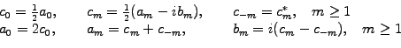
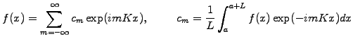
Remember that a complex function of period $L=2\pi/K$ can be represented with a complex series

$\displaystyle f(x)=\sum_{m=-\infty}^\infty c_m \exp(imKx), \hspace{1cm} c_m=\frac{1}{L}\int_a^{a+L} f(x)\exp(-imKx) dx$

(1)

On the other hand, you can use the cosine-sine form

$\displaystyle f(x)=\frac{a_0}{2}+\sum_{m=1}^\infty \left[a_m\cos(mKx) +b_m\sin(mKx)\right]$

(2)

$\displaystyle a_m=\frac{2}{L}\int_a^{a+L} f(x)\cos(mKx) dx \;\;\;(m\ge 0), \hspace{7mm} b_m=\frac{2}{L}\int_a^{a+L} f(x)\sin(mKx) dx \;\;\;(m\ge 1)$

(3)

with the following relations that hold between the Fourier coefficients

$\begin{displaymath}\begin{array}{lll} c_0=\frac{1}{2}a_0, \hspace{5mm} & c_m=\fr... ...m}, \hspace{5mm} & b_m=i(c_m-c_{-m}), \;\;\; m\ge 1 \end{array}\end{displaymath}$

(4)

and only if

is real

$\displaystyle a_0=2c_0, \hspace{5mm} a_m= 2\mathrm{Re}(c_m), \hspace{5mm} b_m=-2\mathrm{Im}(c_m), \hspace{5mm} c_m=c_{-m}^*, \;\;\; m\ge 1$

(5)

This is almost how the transformation has been implemented in FFT.java, except that

The number of modes is assumed to be an integer power of 2; the creation of an FFT-object from data sampled on a mesh therefore relies on the command
```
      double f = new double[64];
      FFT myFTObject = new FFT(f, FFT.inXSpace);
```
where FFT.inXSpace sets the original location of the variable myFTObject in configuration space.

To avoid negative indices for periodic functions

, negative harmonics

are stored in wrap-around order after the positive components and are indexed by

. For a real function $f(x)=[7+8\cos(2\pi x/64)+4\sin(2\pi x/32)+3\cos(2\pi x/2)]$ sampled on a mesh

with a period

, the call to

      Complex spectrum = new Complex[64];
      double periodicity=64.;
      spectrum = myFTObject.getFromKSpace(FFT.firstPart,periodicity);
      for (int m=0;  m<N;  m++) 
         System.out.println("spectrum["+m+"] = "+spectrum[m]);

will print the non-zero components

      spectrum[0] = (7. +0.0i)
      spectrum[1] = (4. +0.0i)          spectrum[63] = (4. +0.0i)
      spectrum[2] = (0. +2.0i)          spectrum[62] = (0. -2.0i)
      spectrum[32]= (3. +0.0i)

It is easy to see that the shortest wavelength component [32] will always be real if

is real, since $\sin(2\pi x/2)$ is sampled exactly for multiples of $\pi$ .

Relying on the linearity of the FFT, two real numbers are packed into one complex number and transformed for the cost of a single complex transformation by initializing
```
      double f = new double[64];
      double g = new double[64];
      FFT myPair = new FFT(f,g, FFT.inXSpace);
```
This is the reason for the argument FFT.firstPart used here above, asking for the spectrum of only the first (and in this example the only) function.

Apart from the array index which starts with [0] in JAVA, the implementation is equivalent to the routines in Numerical Recipes [24] and indeed very similar to that of many computer vendors.

SYLLABUS Previous: 4 FOURIER TRANSFORM Up: 4 FOURIER TRANSFORM Next: 4.2 Linear equations.