

 ','..','$myPermit') ?>
SYLLABUS Previous: 4.2 Linear equations.
Up: 4 FOURIER TRANSFORM
Next: 4.4 Non-linear equations.
','..','$myPermit') ?>
SYLLABUS Previous: 4.2 Linear equations.
Up: 4 FOURIER TRANSFORM
Next: 4.4 Non-linear equations.
4.3 Aliasing, filters and convolution.
Slide : [
Aliasing -
Filters -
Convolution ||
VIDEO
99) echo "
modem -
ISDN -
LAN
"; else echo "login";?>
]
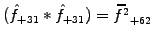
One of the beauties when using Fourier transforms, is the ability to work
with a spectrum of modes and act on each of the components individually
with a filter.
By sampling the function over a period  with a finite number of
values
with a finite number of
values
 , where
  is the size of the sampling interval,
the spectrum gets truncated at the shortest wavelength
is the size of the sampling interval,
the spectrum gets truncated at the shortest wavelength
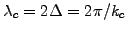 called Nyquist critical wavelength:
this corresponds to exactly 2 mesh points per wavelength, which
does however not mean that shorter wavelengths
called Nyquist critical wavelength:
this corresponds to exactly 2 mesh points per wavelength, which
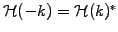
does however not mean that shorter wavelengths  do not
contribute to the Fourier coefficients (4.1#eq.1).
Figure 4.3#fig.1 illustrates how they get aliased back into
the lower components of the spectrum.
do not
contribute to the Fourier coefficients (4.1#eq.1).
Figure 4.3#fig.1 illustrates how they get aliased back into
the lower components of the spectrum.
Figure 4.3#fig.1:
Aliasing from Fourier components shorter than the Nyquist
critical wavelength
.
|
|
This can be important for the digital data acquisition of an experiment,
where the signal has to be low-pass filtered before it is digitally
sampled.
Figure 4.3 shows that even with the greatest precautions,
such an aliasing can sometimes not be avoided, an needs then to be
correctly interpreted.
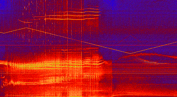
Figure 2:
Experimental spectrum 0-500 kHz digitally recorded during 2 sec from the
magnetic perturbations in a fusion plasma in the
Joint European Torus.
Apart from the Alfvén instabilities which are the subject of this
research, you can see the sawteeth-like trace of an exciter antenna
reaching a minimum of 200 kHz around 1.5 sec; despite heavy analogic
low-pass filtering before the signal is sampled, the large dynamic range
of the measurement above 80 dB is here sensitive enough to pick up
(dark red line) a non-linearly induced high-frequency component which is
aliased down into the frequency range of interest.
Courtesy of
Prof. A. Fasoli(MIT/USA).
|
|
It is easy to design a filter in Fourier space
simply by multiplying the spectrum by a suitable filter function
 (exercise 4.2). Simply remember that
- to keep the data real after transforming back to X-space, you must
keep
 , for example by choosing
 real and even in
  ,
,
- the filter has to be defined in the entire interval
![$ k\in[-k_c;k_c]$](s4img41.gif) and should be smooth to avoid phase errors and dampings for wavelengths
that appear with sharp edges.
and should be smooth to avoid phase errors and dampings for wavelengths
that appear with sharp edges.
Although they are present right from the beginning when the initial
condition is first discretized (try to initialize and propagate an
aliased cosine with ICWavelength=1.05 mesh points per
wavelength using the JBONE applet above), aliases do not
actually interfere with the resolution of linear equations.
The story is however different for spatial non-linearities such as the
quadratic term
 that is responsible for the wave-breaking (1.3.4#eq.1).
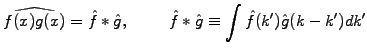
Indeed, think of the convolution theorem, which tells that the
Fourier transform of a convolution
that is responsible for the wave-breaking (1.3.4#eq.1).
Indeed, think of the convolution theorem, which tells that the
Fourier transform of a convolution
 is just the product
of the individual Fourier transforms
is just the product
of the individual Fourier transforms
 . The converse is
unfortunately also true: what can be viewed as a simple product in
X-space becomes a convolution in K-space
. The converse is
unfortunately also true: what can be viewed as a simple product in
X-space becomes a convolution in K-space
 |
(1) |
or in discrete form
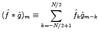 |
(2) |
For the quadratic wave-breaking non-linearity, this shows that a
short wavelength component such as
 in a sampling with
64 points, will incorrectly ``pollute'' a long wavelength channel
through aliasing:
in a sampling with
64 points, will incorrectly ``pollute'' a long wavelength channel
through aliasing:
 .
A simple cure for this, is to expand the size of the arrays by a
factor two before the convolution takes place and pad them with
zeros; changing the representation to calculate the multiplication of
arrays twice the original size, the upper part of the spectrum is
then simply discarded after the data has been transformed back.
The entire procedure is illustrated in the coming section, where
the non-linear Korteweg-DeVries (1.3.4#eq.3) and Burger equations
(1.3.4#eq.2) are solved with a convolution in Fourier space.
.
A simple cure for this, is to expand the size of the arrays by a
factor two before the convolution takes place and pad them with
zeros; changing the representation to calculate the multiplication of
arrays twice the original size, the upper part of the spectrum is
then simply discarded after the data has been transformed back.
The entire procedure is illustrated in the coming section, where
the non-linear Korteweg-DeVries (1.3.4#eq.3) and Burger equations
(1.3.4#eq.2) are solved with a convolution in Fourier space.
SYLLABUS Previous: 4.2 Linear equations.
Up: 4 FOURIER TRANSFORM
Next: 4.4 Non-linear equations.
![\includegraphics[width=10cm]{figs/FFTalias.eps}](s4img36.gif)