Numerical aspects of option pricing : the Black-Scholes equation.
by Christophe Duwig
Introduction :
The most common use of partial differential equation
(pde) is the modelling of dynamic evolution of systems. The governing equations,
often, derives from balance on infinitesimal volumes or variations. Interest
of physicians in solving these equation in so big that there were pioneers
in such area (e.g.. Euler). Today the numerical tools are essential for
the simulation of physical, chemical or biochemical processes. Numeric's
became a branch of science between mathematics and physics.
In these conditions, the knowledge in numeric could
be applied on many system simulations within physics, chemistry, biology,
environmental, financial or social sciences. In this project, the Black-Scholes
equation has been solve. This equation, which looks like any pde of theoretical
physics, describes the evolution of an option price with the exercise price
the time of an asset or financial product whose value is quoted
(see definitions below). This "exotic" application of numerical tool has
been studied and different method has been used to solve the equation.
1. Some elements of financial background
a. Definitions
According to Wilmot et al. (Option Pricing , oxford
financial editions), an European call option could be defined as
a contract which gives the right to his owner to buy at a prescribed time
(expiry date), a prescribed asset (underlying asset) for
a prescribed amount (exercise price). This contract gives a right
to buy the asset but as it's not an obligation, the holder has to buy the
right. The question is then to estimate a correct price of the option in
order to make money in the final transaction (the asset is bought at the
prescribed amount and sold at the current price).
The underlying hypothesis is that the share price
(of the asset) will increase with time (to make profit), the variation
of this price is unknow but it has a influence on the price of the otpions.
Other factors involved are the excercise price (the price the asset may
be bought), the time before expiry, the volatility of the asset
price (which describes stochastic fluctuation in time) and the interset
rate during to following period.
The main constrain in financial application modelling
is the notion of arbitrage. This lead to consider that there is
no possibility to make risk-free profit (guaranteed return) over what could
be obtained by deposing cash in a bank. Further benefits should lead to
take risks.
In fact the Market makers are making profits
by selling above and buying below the price of an asset, the less risk
induced by the option possibility is then attractive for the speculation.
The call otpion has been defined aboveas the right
to buy, another right (the right to sell) is call a put option.
The previous section deals with European option types,
American
options differs in the way that the right may use at any time until
the expiry date. In this case, another question is added : what is the
best moment to act ?
The previous paragraph's purpose was to define
some terms in order to make the background of the equation understandable
but does not pretend to decribe the options' market, further information
about the stock market could be found in Wilmot et al.
b. The Black-Scholes equation.
To derive the Black-Scholes equation, Wilmott et al.
make some assumption about the evolution of the system. The asset price
follows the lognormal random walk, the risk-free rate and the volatility
are known as time functions, the transactions costs are nulls ...
Let V be the option price, E the exercise price, S the asset's price,
s
the volatility of the asset price, t the time, T the expiry time, r the
interest rate and D0 the dividend (here assumed to be null).
Trough a statistical approach of the variation of the asset price for its
random part, the variation of value P of a portfolio
consisting of one option and a well chosen number of the underlying asset
is given by :
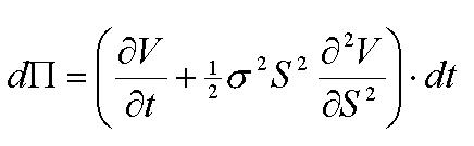 the variation of this portfolio on a riskless account is rPdt
which bounded this variation. By substituing these two expressions,
the Black-Scholes equation is obtained :
the variation of this portfolio on a riskless account is rPdt
which bounded this variation. By substituing these two expressions,
the Black-Scholes equation is obtained :
This equation admit a infinity of solutions since final and boundaries
conditions are not set. It make sense to use the right to buy if at t=T,
S is superior than E (so benefits are made). Final conditions could be
derived from this for the equation in the case of a call option,
V(S,T)=C(S,T)=max(S-E, 0)
in the case of a put option, the condition is,
V(S,T)=P(S,T)=max(-S+E, 0).
For an option call, in the case of S=0, V=C(0,t)=0 and for S
reaching the infinity, V(S,T)~S.
With this conditions, the system is perfectly defined.
For an American option, the allowance to use the
right at any time, will lead to a another condition to avoid risk-free
operation. This condition is :
V(S,T)>=max(S-E, 0)
This kind of constrain is called an obstacle problem.
2. Resolution of the equation.