fd

c. The finite volume approach.

- The reduction of the Black-Scholes equation.

The Black-Scholes equation is given as defined previously :

    The term before the second derivative is positive, formally it lead to a negative diffusion. A steady perturbation, exp(-k*S), will be amplified by the equation an numerical instabilities will result.
    The negative coefficient behind V is also a cause of divergence, lets consider a uniform perturbation, exp(a*t). This equation gives that a=r>0. The perturbation will also be amplified and numerical instabilities could raise. To avoid these problem, the resolution of a modified equation is a elegant way to avoid these problems.
    The finite volume approch will lead to the same scheme as the finite differences by considering the basic diffusion equation. The have a overview of what this method could done, lets consider the original equation. The finite volume discretization consiste of intergrating the pde in the way to have a equation on flux expressions (or with term which could be interpreted as flux). This approach is very popular for CFD applications because through this approach, unstructured mesh could be used which is needed for some applications (as turbomachinery blade oscillations). Before being able to do it, a modification of the Black-Scholes equation is needed in order to eliminate the non constant terms before the derivatives. The resulting equation is :

Using the numerical values given in the exercise 2.5, the coefficient before V is positive so a better stability could be expected during the resolution of this transformed equation. The integration in time will be fully implicit.
Lets consider the control volume around the node i.

In this application, all intervals are supposed having equal lenght, h, and e and w are located in the middle of the interval. The integration on S between w and e gives :

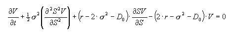
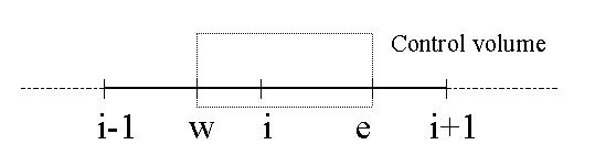
For an implicit approach, V will equal V^t+Dt. The evaluation of the quantities at e and w depends on the scheme. The one choosen for this application in Upwind. For any quantity f, regarding the sign of the tern before the first derivative, we have : f_e=f_i+1 and f_w=f_i.
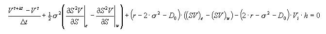
the derivative term is calculated from a first order Taylor expansion serie. Further information could be found in Patankar S. V. 1980. Numerical heat transfer and fluid flow. (Eds. Taylor and Francis)

You can try to run it in the applet below.

align=center width=800 height=280>

Comparison with resolution using a Monte Carlo method is available on this link.

The resulting code, implemented in jbone is given below :

//=======================================================================

// FV Black-Scholes equation

//=======================================================================

BandMatrix a = new BandMatrix(3, f.length);
BandMatrix b = new BandMatrix(3, f.length);
double[] c = new double[f.length];
double[] cst = new double[f.length];
double step=jbone.step;
double sigma = 0.45;
double Dzero = velocity;
double re = 0.1;
double h=dx[0];
double alphabs=re-Dzero-2*sigma*sigma;
double betabs =2*re-sigma*sigma-Dzero;
double moinsdt = timeStep;

for (int i=1; i<=n-1; i++) {
a.setR(i, -(double)(i+1)*(double)(i+1)*sigma*sigma/2*moinsdt- alphabs*(double)(i+1)*moinsdt);
a.setD(i, 1. +sigma*sigma*moinsdt*(double)(i)*(double)(i) +(double)(i)*moinsdt*alphabs- betabs*moinsdt );
a.setL(i, -(double)(i-1)*(double)(i-1)*sigma*sigma/2*moinsdt);
b.setL(i, 0.0 ); //Right hand side
b.setD(i, 1. ); b.setR(i, 0.0 ); } //Matrix elements

// Definition of the boundary conditions
a.setR(0, 0. ); //Matrix elements
a.setD(0, 1. );
a.setL(0, 0. );
b.setL(0, 0. ); //Right hand side
b.setD(0, 0. );
b.setR(0, 0. );
b.setL(n, 0. ); //Right hand side
b.setD(n, 1. );
b.setR(n, 0. );
a.setD(n, 0. );
a.setL(n, 1. );
c=b.dot(f); //Right hand side
c[n]=5.75;
fp=a.solve3(c);

isDefined = true;