','..','$myPermit') ?>
SYLLABUS Previous: 4.1 Plain vanilla stock
Up: 4.1 Plain vanilla stock
Next: 4.1.2 Parameters illustrated with
','..','$myPermit') ?>
SYLLABUS Previous: 4.1 Plain vanilla stock
Up: 4.1 Plain vanilla stock
Next: 4.1.2 Parameters illustrated with
Remember how the price of an option has been calculated in sect.3.1:
with a small twist, this will show you how sophisticated Monte-Carlo
simulations are carried out in practice.
Consider a European call giving its holder the right to buy a share for a
strike of ![]() EUR when the contract expires in 3 months or
EUR when the contract expires in 3 months or ![]() year.
For simplicity, assume that the terminal price of a share presently valued
at
year.
For simplicity, assume that the terminal price of a share presently valued
at ![]() EUR can take only one of two uncertain values with equal
probabilities:
EUR can take only one of two uncertain values with equal
probabilities: ![]() and
and ![]() EUR.
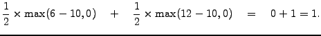
Using this probabilistic knowledge, it is easy to calculate the expected
value at the expiry by weighting the terminal payoff (2.1.3#eq.1)
from each realization with the probability factor 1/2:
EUR.
Using this probabilistic knowledge, it is easy to calculate the expected
value at the expiry by weighting the terminal payoff (2.1.3#eq.1)
from each realization with the probability factor 1/2:
Even if the principle is correct, we showed in sect.3.2 that
the forecasting values (3.2#eq.4) have to be carefully chosen to
reproduce the market volatility, for example 40% (
![]() ):
this yields
):
this yields
![]() and
risk-neutral world probabilities (3.2#eq.3) where a movement up
and
risk-neutral world probabilities (3.2#eq.3) where a movement up
![]() is slightly less
likely than a movement down
is slightly less
likely than a movement down
![]() .
These parameters can again be used to calculate the expected payoff for
different market values of the underlying share
.
These parameters can again be used to calculate the expected payoff for
different market values of the underlying share ![]()
|
Almost the same procedure is used in a Monte-Carlo calculation, except
that for a higher accuracy, the lifetime of the option is divided into
smaller steps:
increments are accumulated to simulate possible realizations
starting from the initial (spot) price of the underlying
(log-normal walk with shares
in sect.2.1.1) and set the drift equal to the spot rate
(risk-neutral evolution observed
for trees in sect.3.2).
After each time step, the arithmetic average from all the possible
terminal payoffs is used to estimate the mean price of the option
on the expiring date and is discounted back in time to plot the
fair value of an option having a lifetime equal to the run time.
The VMARKET applet below
shows an example with (Volatility=0.4, Drift=0.03), where
new increments are generated every trading day (the duration of one
step is ![]() =1/252=0.00397 year) and are accumulated to forecast
two possible realizations of the underlying spot price (
=1/252=0.00397 year) and are accumulated to forecast
two possible realizations of the underlying spot price (![]() , red dots)
starting from an initial 10 EUR (coincides with the StrikePrice).
After one step backward in time (
, red dots)
starting from an initial 10 EUR (coincides with the StrikePrice).
After one step backward in time (
![]() or Time=0.003 displayed
on the top of the applet measures the lifetime ranging from
or Time=0.003 displayed
on the top of the applet measures the lifetime ranging from ![]() to
to ![]() ),
the fair value of the option
),
the fair value of the option
![]() is plotted (in black)
together with the terminal payoff
is plotted (in black)
together with the terminal payoff ![]() (in grey).
Running the simulation for 3 months (Time=0.25), the prices
obtained using the Monte-Carlo method can be cross-checked with the
value obtained from the binomial step (4.1.1#tab.1): they are quite
different!
(in grey).
Running the simulation for 3 months (Time=0.25), the prices
obtained using the Monte-Carlo method can be cross-checked with the
value obtained from the binomial step (4.1.1#tab.1): they are quite
different!
The experiments show that the numerical accuracy of the Monte-Carlo
calculation can be improved by increasing the number of realizations:
the values obtained approach those given in (4.1.1#tab.1) without
reproducing them exactly. The difference is particularly striking for
low values of the underlying ![]() , where the binomial step gives
options that are worthless, while the Monte-Carlo method converges to
small but finite values.
As you may have guessed, also binomial trees are only an approximation
of the true solution, with an accuracy that improves when the number of
steps is increased-resulting in a larger number of forecasting prices.
As a matter of fact, both methods converge to the same value in the
limit of small time steps and a large number of realisations: this
value is the same as the one that has first been obtained by
Black & Scholes [3] by solving (3.4#eq.4).
, where the binomial step gives
options that are worthless, while the Monte-Carlo method converges to
small but finite values.
As you may have guessed, also binomial trees are only an approximation
of the true solution, with an accuracy that improves when the number of
steps is increased-resulting in a larger number of forecasting prices.
As a matter of fact, both methods converge to the same value in the
limit of small time steps and a large number of realisations: this
value is the same as the one that has first been obtained by
Black & Scholes [3] by solving (3.4#eq.4).
Congratulations: you probably solved your first option pricing equation and hopefully even understood what you were doing! Of course, analytical minded persons may say that a formula is more general and provides a better understanding. In this syllabus, we argue the opposite: formulas, just like computers, are only tools to obtain solutions from a certain model of the reality. Analytical and computational tools are both perfectly adequate if they are used in a knowledgable manner: they are often favourably compared to ensure that the solution is not affected by different assumptions made during the derivation of the models.
Before tackling these issues, let us first develop an intuition for the financial parameters and study with experiments how they affect the option payoff before the expiry date.
SYLLABUS Previous: 4.1 Plain vanilla stock Up: 4.1 Plain vanilla stock Next: 4.1.2 Parameters illustrated with