

 SYLLABUS Previous: 2.2.1 Interest rates: treasury
Up: 2.2 The credit market
Next: 2.2.3 Interest rate swaps
SYLLABUS Previous: 2.2.1 Interest rates: treasury
Up: 2.2 The credit market
Next: 2.2.3 Interest rate swaps
2.2.2 Underlying discount bonds and forward rates

[ SLIDE
discount bond -
spot rate -
forward rate || same
VIDEO as previous section:
modem -
LAN -
DSL ]
The introductory section 1.3 suggested how fixed income
securities, which pay a stream of coupons some time in the future ti>t
are a form of contingent claim that can always be replicated with a
combination of zero-coupon bonds AP(t,ti).
Rather than the interest rate, it is the present value of such zero-coupon
bonds that is traded on the bond market, with a spot price for each maturity
date that is determined by the offer and demand from the investors.
Given the similarity with the stock market, it is not surprising that most
of the derivatives that have been discussed for shares can be generalized
for bonds.
For simplicity, the principal is often normalized to unity A=1
and the
discount bond P(t,T)
is used as a building block for more elaborate products.
The discount function P(0,T)
in particular measures the present value of one unit due at a later time T;
(2.2.2#fig.1) shows an example at a time when the treasury rate was
relatively low and the market expects rising interest rates.
Figure 2.2.2#fig.1:
On the left, a discount function  from the market with up to
 years maturity; on the right the corresponding zero-yield rates
using a simple
years maturity; on the right the corresponding zero-yield rates
using a simple  (line) and a discrete one year compounding
 (dashes) together with the one year forward rates
 (dots).
|
|
For a short time, the spot rate r(t)
taken e.g. from the inter-bank market is nearly constant and the yield
can be calculated without compounding Rs(t,T)
in (2.2.2#eq.1, left). For longer periods, a compounded calculation
has to be used Rm(t,T)
in (2.2.2#eq.1, right) and is often replaced by a continuous compounding
with a rate R(t,T)=exp[Y(t,T)]-1
calculated from the discount factor (2.2.2#eq.1, bottom)
![$\displaystyle P(t,T)=\exp[-Y(t,T)(T-t)]$](s2img97.gif) |
(2.2.2#eq.1) |
Plotted as a function of the time to maturity R(0,T),
these yield curves are often called the
term structure of interest rates
and can directly be constructed from the price of discount bonds
quoted on the market (2.2.2#fig.1, 2.2.2#tab.1, exercise 2.09).
Depending on whether the treasury rate is below or above the market
expectations for the longer term interest rates, the term structure
can have either a positive slope (as in fig.2.2.2#fig.1, right) or
a negative slope.
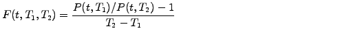
From the ratio between values of the discount function in the future,
it is convenient to define the implied
forward rates,
which correspond to the interest payed today (or any time t<T1<T2)
for a discount bond with a maturity T2
and starting in the future T1
![$\displaystyle F(t,T,T+\Delta t)=-\frac{\ln[P(t,T+\Delta t)/P(t,T)]}{\Delta t}$](s2img99.gif) |
(2.2.2#eq.2) |
As expected, this definition recovers the present value for F(t,t,T)= R(t,T).
Examples of forward rates starting after a delay  are displayed
in (2.2.2#fig.2) and have been derived from the same discount
function that was used previously in (2.2.2#fig.1, 2.2.2#tab.1).
are displayed
in (2.2.2#fig.2) and have been derived from the same discount
function that was used previously in (2.2.2#fig.1, 2.2.2#tab.1).
Figure 2.2.2#fig.2:
Forward rates  starting after a delay
plotted as a
function of the time to maturity
starting after a delay
plotted as a
function of the time to maturity  .
.
|
|
Table 2.2.2#tab.1:
Example of a discount function
and the corresponding
present  and forward rates
starting after a delay
for a maturity date
.
and forward rates
starting after a delay
for a maturity date
.
|
T [years] |
 (0,T)
(0,T) |
 (0,T)
(0,T) |
 (0,T)
(0,T) |
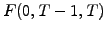
 (0,T-1,T)
 |
(0,1,T) |
(0,2,T) |
(0,3,T) |
|
1 |
0.9662 |
0.0350 |
0.0350 |
0.0350 |
- |
- |
- |
|
2 |
0.9153 |
0.0450 |
0.0452 |
0.0556 |
0.0556 |
- |
- |
|
3 |
0.8563 |
0.0525 |
0.0531 |
0.0690 |
0.0620 |
0.0690 |
- |
|
4 |
0.7947 |
0.0581 |
0.0591 |
0.0775 |
0.0668 |
0.0731 |
0.0775 |
|
5 |
0.7340 |
0.0623 |
0.0638 |
0.0826 |
0.0703 |
0.0760 |
0.0800 |
|
6 |
0.6762 |
0.0655 |
0.0674 |
0.0855 |
0.0729 |
0.0781 |
0.0817 |
|
7 |
0.6222 |
0.0679 |
0.0701 |
0.0867 |
0.0748 |
0.0796 |
0.0828 |
|
8 |
0.5725 |
0.0697 |
0.0722 |
0.0870 |
0.0761 |
0.0806 |
0.0835 |
|
9 |
0.5269 |
0.0710 |
0.0738 |
0.0865 |
0.0771 |
0.0812 |
0.0839 |
|
10 |
0.4853 |
0.0720 |
0.0750 |
0.0857 |
0.0778 |
0.0816 |
0.0841 |
|
Because of the uncertainty associated with the credit worthiness of
long term borrowers and the seemingly random changes of the central
bank policies, the price of a discount bond P(t,T), the yield Y(t,T)
and the forward rates F(t,T1,T2)
are all random functions of time via the spot rate r(t)
which will be discussed further in chapter 3.
Nevertheless, is it possible for loan takers to protect themselves
against unpredictable changes in the interest rate? Yes, using the
so-called swaps and forward rate agreements.
SYLLABUS Previous: 2.2.1 Interest rates: treasury
Up: 2.2 The credit market
Next: 2.2.3 Interest rate swaps
![\includegraphics[width=7cm]{figs/discount.eps}](s2img94.gif)
![\includegraphics[width=7cm]{figs/rates.eps}](s2img95.gif)
![$\displaystyle P(t,T)=\frac{1}{1+R_s(t,T)(T-t)} \hspace{1cm} P(t,T)=\frac{1}{[1+R_m(t,T)/m]^{T-t}}$](s2img96.gif)
![\includegraphics[width=7cm]{figs/ratesFwd.eps}](s2img100.gif)