

 ','..','$myPermit') ?>
SYLLABUS Previous: 1.3 Prototype problems
Up: 1.3 Prototype problems
Next: 1.3.2 Diffusion
','..','$myPermit') ?>
SYLLABUS Previous: 1.3 Prototype problems
Up: 1.3 Prototype problems
Next: 1.3.2 Diffusion
1.3.1 Advection
Slide : [
advection -
waves ||
VIDEO
99) echo "
modem -
ISDN -
LAN
"; else echo "login";?>
]
Also called convection, advection models the streaming of
infinitesimal elements in a fluid. It generally appears when a transport
process is modeled in a Eulerian representation using the convective
derivative
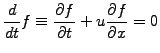 |
(1.3.1#eq.1) |
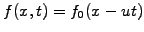
For a constant advection velocity  , the advection equation can be
solved analytically
, the advection equation can be
solved analytically
 ,
showing explicitly the underlying characteristic
,
showing explicitly the underlying characteristic  .
Try the JBONE applet
below
to compute the advection of a Gaussian pulse using the Lagrangian CIP
method from chapter 6.
.
Try the JBONE applet
below
to compute the advection of a Gaussian pulse using the Lagrangian CIP
method from chapter 6.
JBONE applet: press Start/Stop
to simulate the advection of a Gaussian pulse.
Verify that the pulse indeed propagates with an advection velocity
u=1 as chosen in the input parameters.
|
|
"; ?>
Both experiments show that numerical simulations have to be used carefully,
to work withing limits of applicability that will be discussed in the
comming sections.
Note that for a constant advection speed, the wave equation can be written
in flux-conservative form that reminds an advection
![$\displaystyle \frac{\partial^2 h}{\partial t^2} -u^2 \frac{\partial^2 h}{\parti...
...}\right)\cdot \left(\begin{array}{c}\!\!f\\ \!\!g \end{array}\right) \right] =0$](s1img81.gif) |
(1.3.1#eq.2) |
This shows explicitly that the numerical methods for the advection
equation can in principle be used also for wave problems.
SYLLABUS Previous: 1.3 Prototype problems
Up: 1.3 Prototype problems
Next: 1.3.2 Diffusion