3.6 Variational inequalities

SYLLABUS Previous: 3.5 Linear solvers Up: 3 FINITE ELEMENT METHOD Next: 3.7 Computer quiz

3.6 Variational inequalities

Slide : [ obstacle problem - complementarity form - variational form || VIDEO login]

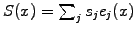
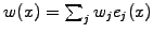
Consider the simplest obstacle problem, which arises when an elastic string held fixed at both ends is pulled over a smooth object and an equilibrium is sought without knowing a priori where are the regions of contact between the string and this object. Define the function $S(x)\in\mathcal{C}^1(\Omega)$ measuring the elevation of the string in the interval $\Omega=[x_L;x_R]$ and the function $O(x)\in\mathcal{C}^1(\Omega)$ modeling the shape of the object.

Mathematically, the obstacle problem amounts to finding a solution satisfying the conditions:

the string always remains above the obstacle $S(x)\ge O(x)$ ,
the string satisfies the equilibrium equation. Neglecting the inertia, this says that the string has either zero curvature (straight line between the points of contact) or a negative curvature $S^{\prime\prime}\le 0$ (line of contact - in other words, the obstacle can only push the string up, not pull it down).

This section considers two methods for solving problems that involve inequalities.

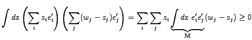
Linear complementary formulation.

Reassemble all the constraints in a form

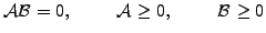$\displaystyle \mathcal{A}\mathcal{B}=0, \hspace{1cm} \mathcal{A}\ge 0, \hspace{1cm} \mathcal{B}\ge 0$

(1)

After discretization, assuming $\mathbf{A}$ invertible and positive definite, the linear problem

$\displaystyle (\mathbf{x}-\mathbf{c})(\mathbf{A}\mathbf{x}-\mathbf{b})=0, \hspace{1cm} \mathbf{A}\mathbf{x}\ge\mathbf{b}, \hspace{1cm} \mathbf{x}\ge\mathbf{c}$

(2)

can be solved with the so-called projected SOR method, by replacing (3.5#eq.10) with

$\displaystyle \mathbf{x_{k+1}} = \max[\mathbf{c}, \omega \mathbf{x_{k}^{GS}} +(1-\omega) \mathbf{x_{k}} ]$

(3)

and making sure that the iteration starts from an initial guess $\mathbf{x_0}\ge\mathbf{c}$ .

For the obstacle problem, the string follows either a straight line above the obstacle $S^{\prime\prime}=0$ or fits exactly the object ; this leads to a complementary problem

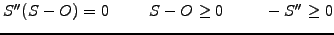$\displaystyle S^{\prime\prime}(S-O)=0 \hspace{1cm} S-O\ge 0 \hspace{1cm} -S^{\prime\prime}\ge 0$

(4)

which be discretized using finite differences and solved with the projected SOR method (exercise 3.05).

Variational formulation.

This approach is particularly well suited for a discretization with finite elements is and best illustrated directly with the example. Choose a test function 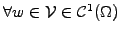$\forall w\in\mathcal{V}\in\mathcal{C}^1(\Omega)$ that satisfies the same constraints as the solution $(w-c)\ge 0$ . Having already $(S-c)\ge 0$ and $-S^{\prime\prime}\ge 0$ , write two inequalities

$\displaystyle \int_{x_L}^{x_R} -S^{\prime\prime}(w-c)\ge 0$
$\displaystyle \int_{x_L}^{x_R} -S^{\prime\prime}(S-c)\ge 0$

and subtract them

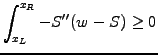$\displaystyle \int_{x_L}^{x_R} -S^{\prime\prime}(w-S)\ge 0$

(5)

The constraint

now appears only implicitly through the fact that

and

are members of the same sub-space $\mathcal{V}$ ; all what remains to be done is to prove that the inequality (3.6#eq.5) in fact is a strict equality if the solution satisfies the constraint. After integration by parts and discretization with linear FEMs, the problem can therefore be solved with projected SOR iterations (3.6#eq.3, exercises 3.05 and 3.07).

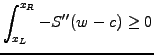
To prove that (3.6#eq.5) satisfies a strict equality, integrate by part and a discretize $S(x)=\sum_j s_j e_j(x)$ and $w(x)=\sum_j w_j e_j(x)$ with linear finite elements

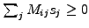
$\displaystyle \int dx \left(\sum_i s_i e_i^\prime\right) \left(\sum_j (w_j-s_j)... ...m_j s_i \underbrace{\int dx \; e_i^\prime e_j^\prime}_\mathbf{M}(w_j-s_j) \ge 0$

If the matrix is symmetric $\mathbf{M^T}=\mathbf{M}$ as is the case with diffusion, this simply yields

$\displaystyle \mathbf{s^T M (w-s)} = \mathbf{(w-s)^T M^T s} = \mathbf{(w-s)^T M s} \ge 0$

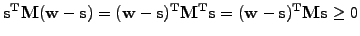(6)

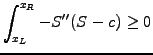
If the problem is positive definite $\sum_j M_{ij} s_j\ge 0$ as is the case with diffusion and the solution satisfies the constraint $s_i-c_i\ge 0$ , the product satisfies the inequality

$\displaystyle \mathbf{(s-c)^T M s} \ge 0$

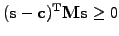(7)

Since (3.6#eq.6) must hold for the particular choice where the test function coincides with the constraint $\mathbf{w}=\mathbf{c}$ , the last two inequalities can only be satisfied simultaneously if they both satisfy the strict equality. $\square$

SYLLABUS Previous: 3.5 Linear solvers Up: 3 FINITE ELEMENT METHOD Next: 3.7 Computer quiz