2.4 Leap-frog, staggered grids

SYLLABUS Previous: 2.3 Lax-Wendroff Up: 2 FINITE DIFFERENCES Next: 2.5 Implicit Crank-Nicholson

2.4 Leap-frog, staggered grids

Slide : [ Staggered leapfrog Scheme - Code - Run || VIDEO login]

The leap-frog algorithm is often used for the propagation of waves, where a low numerical damping is required with a relatively high accuracy. Relying on two functions $\{f,g\}$ to approximate the scalar wave equation (1.3.1#eq.2) in flux-conservative form, staggered grids (where the mesh points are shifted with respect to each other by half an interval, as in fig.2.4#fig.4) are used to evaluate centered differences with an accuracy in $\mathcal{O}(\Delta x^2 \Delta t^2)$ :

**Figure 2.4#fig.4:** Staggered grids.
$\includegraphics[width=5cm]{figs/FDeStag.eps}$

$\displaystyle \left\{\begin{array}{l} \frac{1}{\Delta t} \left[f_{j+1/2}^{t+\De... ...frac{u}{\Delta x} \left[f_{j+1/2}^{t }-f_{j-1/2}^{t }\right] \end{array}\right.$

(2.4.0#eq.9)

The construction of the leap-frog algorithm suggests how the Maxwell equations can be discretized using finite differences in the time domain (FDTD) to solve vector equations in terms of the electric and the magnetic fields evaluated on staggered grids (exercise 2.08). The leap-frog algorithm has been implemented in JBONE as

      for (int j=1; j<=n; j++) {                  //1st equation
        fp[j]=f[j] -beta*(g[j]-g[j-1]); }
      fp[0]=f[0] -beta*(g[0]-g[n]);
      for (int j=0; j<=n-1; j++) {                //2nd equation
        gp[j]=g[j] -beta*(fp[j+1]-fp[j]); }
      gp[n]=g[n] -beta*(fp[0]-fp[n]);

Special care is required when starting the integration, since the initial condition $g_j^{-\Delta t/2}$ determines the direction of propagation (exercise 2.04). In addition to the periodic boundaries shown here above, Dirichlet and absorbing boundary conditions are also frequently used (exercises 2.04 and 2.08).

**JBONE applet:** press **Start/Stop** to simulate the propagation a scalar wave in a periodic domain using two functions f (in black) and g (in blue).

Numerical experiments: leap-frog

Examine the propagation and the damping of harmonic functions; try to assess the numerical properties directly from your observations.

Study the initialization with PhysDataValue in .

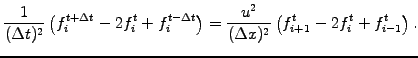
By substitution, note that the leap-frog scheme is equivalent to the implicit 3 levels scheme

$\displaystyle \frac{ 1 }{(\Delta t)^2} \left(f_i^{t+\Delta t} -2f_i^t +f_i^{t-\... ...t}\right)= \frac{u^2}{(\Delta x)^2} \left(f_{i+1}^t -2f_i^t +f_{i-1}^t\right) .$

(2.4.0#eq.10)

where the linear problem has been solved explicitly in an elegant manner.

SYLLABUS Previous: 2.3 Lax-Wendroff Up: 2 FINITE DIFFERENCES Next: 2.5 Implicit Crank-Nicholson