4.2 Linear equations.

SYLLABUS Previous: 4.1 FFT with the Up: 4 FOURIER TRANSFORM Next: 4.3 Aliasing, filters and

4.2 Linear equations.

Slide : [ Scheme - Code - Run || VIDEO login]

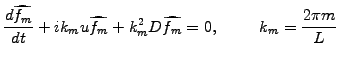
Albeit slower, with $\mathcal{O}(N\log N)$ operations per time-step, than the numerical schemes in $\mathcal{O}(N)$ we have seen so far, FFTs can be used to compute the Fourier representation of the advection-diffusion problem (1.3.2#eq.2) and describe the evolution of each Fourier component separately

$\displaystyle \frac{d \widehat{f_m}}{dt} +ik_mu \widehat{f_m} +k_m^2D \widehat{f_m} = 0, \hspace{1cm}k_m=\frac{2\pi m}{L}$

(1)

The equation can be integrated analytically without any restriction on the time-step; starting directly from the initial condition, this yields for each Fourier component

$\displaystyle \widehat{f_m}(t)=\widehat{f_m}(0)\exp[-(ik_mu +k_m^2D)t)]$

(2)

After the initialization, where the initial condition is discretized by sampling on a regular mesh and stored for subsequent transformation, the scheme implemented in JBONE reads:

      int N         = mesh_.size();                      //A power of 2
      double boxLen = mesh_.size()*mesh_.interval(0);    //Periodicity
      double   k    = 2*Math.PI/boxLen;                  //Notation
      Complex ik1   = new Complex(  0.,  k  );
      Complex ik2   = new Complex(-k*k,  0.  );

      Complex advection = new Complex(ik1.scale(velocity));  //Variables
      Complex diffusion = new Complex(ik2.scale(diffusCo));

      Complex[] s0 = new Complex[f.length];              //FFT real to KSpace
      s0=keepFFT.getFromKSpace(FFT.firstPart,boxLen);    //  only once
                                                         
      s[0] = s0[0];
      for (int m=1;  m<N/2+1;  m++) {                    //Propagate directly
        total=          advection.scale((double)(m ));   //  from initial
        total=total.add(diffusion.scale((double)(m*m))); //  condition

        exp=(total.scale(timeStep*(double)(jbone.step))).exp();

        s[m  ] = s0[m].mul(exp);                         //  s0 contains the IC
        s[N-m] = s[m].conj();                            //  f is real
      }
      FFT ffts = new FFT(s,FFT.inKSpace);                //Initialize in Kspace
      f = ffts.getFromXSpacePart(FFT.firstPart,boxLen);  //FFT real back for plot

If you read carefully, you probably wonder now about the sign of the phase factor, which is opposite from (4.2#eq.2); the reason is that the phase chosen here for the spatial harmonics is exactly opposite to the one that has been assumed in the FFT routine from Numerical Recipes [24]. This makes the scheme look like as if it evolves backwards in time - it doesn't! Also note that once the initial condition has been transformed to K-space, subsequent transformations back to X-space are in fact only required for plotting.

The example below illustrates the advection of a box calculated with the same time step $\Delta t=0.5$ as previously.

**JBONE applet:** press **Start/Stop** to simulate the advection of a box function, showing what appears to be a perfect solution that alternates with a strong Gibbs phenomenon. In fact, the oscillations are always present in the solution, but disappear from the plot when straight lines are used to connect adjacent mesh points.

The Gibbs phenomenon (an artifact from using harmonic functions for the discretization of sharp edges discussed in sect.1.4.5) is clearly visible except when $u\Delta t/\Delta x$ is an integer; but don't be fooled by the plot routine, which (for simplicity, but still incorrectly) draws straight lines between the grid points when it should in fact draw the complete oscillations that are visible in figure 1.4.5#fig.1. The power of the method is evident when taking large time-steps: edit the parameter to TimeStep=64, add some diffusion Diffusion=0.3 and compare the solution obtained with a single step with the result computed using your favorite FD or FEM scheme from the previous sections²⁰. This is very nice indeed, but remember that dealing with an inhomogeneous medium

or complicated boundary conditions is problematic in Fourier space.

Numerical experiments: linear equations with FFT

Reduce TimeStep=0.1 and observe how the Gibbs phenomenon appears when the position of the box does not exactly coincide with the mesh points chosen for the plot.

Switch to Finite Differences and Finite Elements to measure the quality of previous schemes for Velocity=1, Diffusion=0.5 by comparing the results with the exact solution obtained with the Fourier transform. Hint: re-select the method that is currently being used to re-scale the plot window and monitor Min / Max at the end of the evolution.

Initialize a Gaussian and determine the optimal numerical parameters (MeshPoints, TimeStep, TimeImplicit, TuneIntegr) for different schemes to achieve a 2% precision in the final value of the peak.

SYLLABUS Previous: 4.1 FFT with the Up: 4 FOURIER TRANSFORM Next: 4.3 Aliasing, filters and