

 SYLLABUS Previous: 5.3 Methods for bonds
Up: 5.3 Methods for bonds
Next: 5.3.2 Extensions for derivatives
SYLLABUS Previous: 5.3 Methods for bonds
Up: 5.3 Methods for bonds
Next: 5.3.2 Extensions for derivatives
5.3.1 The Vasicek model for a bond

[ SLIDE
variational form -
implicit time -
FEM -
code -
run ||
VIDEO modem (
1/
2 ) - LAN (
1/
2 ) - DSL (
1/
2)]
The
finite element method
offers considerable advantages in terms of flexibility and robustness at
the expense of a slightly more complicated formulation. For example,
the FEM method does not suffer from the numerical instability
that limits the time stepping in finite difference schemes,
it converges very quickly
in comparison with the Monte-Carlo method using only few driving factors
and the next chapter will show how
the formulation can easily be extended to deal with the American exercise style.
Here we use the Vasicek equation (3.5#eq.6) only to illustrate one
implementation and justify the VMARKET solution for the price of
a bond  as a function of the spot rate and time.
More details about the finite element method and its formulation can be found
on-line.
as a function of the spot rate and time.
More details about the finite element method and its formulation can be found
on-line.
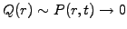
Since the random increments of interest rates are normally distributed in
the Vasicek model, there is no real advantage to transform the problem
into normalized variables. We therefore start directly from the
partial differential equation (3.5#eq.6)
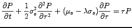
Multiply by an arbitrary test function  , integrate over the
domain
, integrate over the
domain
![$ \Omega=[r_-;r_+]$](s5img90.gif) where the solution is sought and formulate a
variational principle
where the solution is sought and formulate a
variational principle
![$\displaystyle \int_{r_-}^{r_+} dr Q \left[ \frac{\partial P}{\partial t} +\frac...
...tial P}{\partial r} - rP \right] = 0 \qquad \forall Q \in \mathcal{C}^1(\Omega)$](s5img91.gif) |
(5.3.1#eq.1) |
It turns out that this variational problem is equivalent to the original
equation provided that the equation is satisfied for all the test functions
that are ``sufficiently general''.
Galerkin's method of choosing the same functional space as the solution is
an excellent starting point: here it is sufficient to keep piecewise linear
function
 . Indeed, after integration by parts of the
second order term
. Indeed, after integration by parts of the
second order term
 |
(5.3.1#eq.2) |
only first order derivatives remain, which can be evaluated using linear
functions. The surface term that has been produced is used to impose
so-called natural boundary conditions:
the contribution from the upper boundary vanishes if  is large
enough, since
is large
enough, since
 for
for
 when
when  are chosen from the same functional space.
Essential boundary conditions will be
imposed on the lower boundary to normalized the discount function
where
are chosen from the same functional space.
Essential boundary conditions will be
imposed on the lower boundary to normalized the discount function
where  is small, so that the surface term can here simply be
neglected.
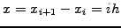
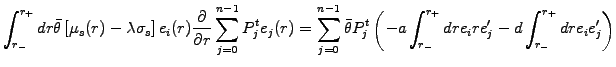
Now discretize the time into small steps using a backward difference for
the first term and a partly implicit evaluation for the rest
is small, so that the surface term can here simply be
neglected.
Now discretize the time into small steps using a backward difference for
the first term and a partly implicit evaluation for the rest
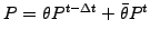 where
where
![$ \theta=1-\bar{\theta}\in[1/2; 1]$](s5img100.gif)
Discretize the interest rates, decomposing the solution into the weighted
sum of finite elements roof-top functions suggested in (5.3.1#fig.1).
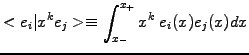
Reassemble dependencies on  into overlap integrals of the form
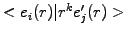 , which can be calculated analytically for
a homogeneous mesh.
Assuming a constant volatility
, which can be calculated analytically for
a homogeneous mesh.
Assuming a constant volatility
 in (3.5#eq.7)
and drift of the form
in (3.5#eq.7)
and drift of the form
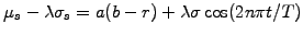 ,
the second last term is conveniently re-written using the coefficient
,
the second last term is conveniently re-written using the coefficient
 as
as
Multiply by  and write all the unknown
 as a function of the known values
To complete the formulation, the problem has to be supplemented with a
terminal condition: from the definition of the discount function
(2.2.2#eq.1) this is
 when
when  .
Boundary conditions have to be justified from no-arbitrage considerations:
for simplicity, the yield in
.
Boundary conditions have to be justified from no-arbitrage considerations:
for simplicity, the yield in
![$ P(0,t)=\exp[-Y(t,T)(T-t)]$](s5img117.gif) (2.2.2#eq.1)
is here somewhat artificially associated with the spot rate and forced to
zero with the Dirichlet condition
(2.2.2#eq.1)
is here somewhat artificially associated with the spot rate and forced to
zero with the Dirichlet condition
 .
A similar reasoning justifies the Neuman condition
.
A similar reasoning justifies the Neuman condition
 and is here implemented for a homogeneous grid
  using the second
order finite difference approximation
using the second
order finite difference approximation
![$ \partial_r P(r_n)\approx[3P(r_n) -4P(r_{n-1})+P(r_{n-2})]/2h$](s5img121.gif) [1].
[1].
Because of the finite extension of finite element roof-top functions
overlapping only with the nearest neighbors, the linear system of
equations (5.3.1#eq.4) can be cast into
 |
(5.3.1#eq.5) |
The matrix  is tridiagonal of the form
 , except
the last row, where an element created by the Neuman condition
, except
the last row, where an element created by the Neuman condition
 has to be eliminated by hand (row
  minus
minus  times row
  ) to
preserve the structure of the matrix
) to
preserve the structure of the matrix
 |
(5.3.1#eq.6) |
After substituting the value for
 and replacing the
last equation by (5.3.1#eq.6), the linear system is solved using standard
LU factorization.
and replacing the
last equation by (5.3.1#eq.6), the linear system is solved using standard
LU factorization.
Quants: linear Galerkin finite element (FEM) discretization.
Decompose the solution  into a superposition of finite element roof-top
functions
into a superposition of finite element roof-top
functions
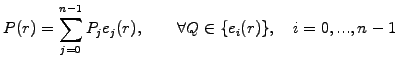 |
(5.3.1#eq.7) |
choosing the same elements for the test function  to create as many
equations as unknowns.
to create as many
equations as unknowns.
Figure 5.3.1#fig.1:
Linear FEM approximation illustrated with a homogeneous mesh.
|
|
Only the nearest neighbors contribute to the overlap integrals; these
can be evaluated with a combination of the trapezoidal and the mid-point
rule
![$\displaystyle \int_{x_i}^{x_{i+1}} f(y) dy \approx (x_{i+1}-x_i)\left[\frac{p}{...
...eft[f(x_i)+f(x_{i+1})\right] + (1-p) f\left(\frac{x_i+x_{i+1}}{2}\right)\right]$](s5img137.gif) |
(5.3.1#eq.9) |
where a suitable choice of the tunable integration parameter
reproduces piecewise constant ( ) or linear FEM approximations
(
) or linear FEM approximations
( ) or the Crank-Nicholson method (
 ).
For a homogeneous mesh
).
For a homogeneous mesh
 , the overlap integrals can be
calculated analytically and the finite contributions yield
, the overlap integrals can be
calculated analytically and the finite contributions yield
 |
(5.3.1#eq.10) |
Despite the rather sophisticated derivation, this finally yields a
very elegant scheme that has been implemented in the VMARKET class
FEMSolution.java
as
      double twopi    = 8.*Math.atan(1.);
      double runTime  = runData.getParamValue("RunTime");
      double timeStep = runData.getParamValue("TimeStep");
      double sigma    = runData.getParamValue("Volatility");
      double theta    = runData.getParamValue("TimeTheta");
      double tune     = runData.getParamValue("TuneQuad");
      double lambda   = runData.getParamValue("MktPriceRsk");
      double t        = 1.-time/runTime;               // normalized time
      double hump     = 1.7*(t-t*t*t*t*t*t);           // volatility shaping
      double ca       = runData.getParamValue(runData.meanRevVeloNm);
      double cb       = runData.getParamValue(runData.meanRevTargNm);
      double cycles   = runData.getParamValue(runData.userDoubleNm);
      double cd       = ca*cb-lambda*sigma*Math.cos(twopi*cycles*t);
      double ce       = sigma*hump; ce=ce*ce;
                                                       //--- CONSTRUCT MATRICES
      BandMatrix a = new BandMatrix(3, f.length);      // Linear problem
      BandMatrix b = new BandMatrix(3, f.length);      //  a*fp=b*f=c
      double[]   c = new double[f.length];
                                                       // Quadrature coeff
      double h,h0,h0o,h1,h1m,h1p,h2,h2o;               //  independent of i
      double t0,t0m,t0p,t1,t1m,t1p;                    //  depending on i
      h= dx[0];
      h0o= 0.25*h*(1-tune);               h0= 0.5*h*(1+tune);
      h1m=-0.5; h1p=-h1m;                 h1= 0.;
      h2o=-1./h;                          h2= 2./h;
      for (int i=0; i<=n; i++) {
        t0m=h*h*0.125*(1-tune)*(2*i-1);
        t0p=h*h*0.125*(1-tune)*(2*i+1);   t0=h*h*0.5*i*(tune+1);
        t1m=h*h*0.25*(-2*i-tune+1);
        t1p=h*h*0.25*(-2*i+tune+1);       t1=h*h*0.5*(tune-1);
        a.setL(i,h0o + theta   *timeStep*(t0m +0.5*ce*h2o +ca*t1m +cd*h1m));
        a.setD(i,h0  + theta   *timeStep*(t0  +0.5*ce*h2  +ca*t1  +cd*h1 ));
        a.setR(i,h0o + theta   *timeStep*(t0p +0.5*ce*h2o +ca*t1p +cd*h1p));
        b.setL(i,h0o +(theta-1)*timeStep*(t0m +0.5*ce*h2o +ca*t1m +cd*h1m));
        b.setD(i,h0  +(theta-1)*timeStep*(t0  +0.5*ce*h2  +ca*t1  +cd*h1 ));
        b.setR(i,h0o +(theta-1)*timeStep*(t0p +0.5*ce*h2o +ca*t1p +cd*h1p));
      }
      c=b.dot(f);
      double dPdy0, dPdyn, c0, cn;                     //--- BC
      a.setL(0, 0.);a.setD(0, 1.);a.setR(0, 0.);c[0]=1.;//left: Dirichlet
      double a1n= a.getD(n-1) +4.*a.getL(n-1);         // right: Neuman
      double ann= a.getR(n-1) -3.*a.getL(n-1);         //   O(h^2)
      dPdyn=-time*f[n]; cn=c[n-1]-2*dx[0]*a.getL(n-1)*dPdyn;
      a.setL(n,a1n);a.setD(n,ann);a.setR(n, 0.);c[n]=cn;
      fp=a.solve3(c);                                  //--- SOLVE
      for (int i=0; i<=n; i++) {                       //--- PLOT
        gp[i]=-Math.log(fp[i])/time;                   // yield(r)
        if (time<=timeStep) f0[i]=0.;
      }
      int i=(int)((time/runTime*n));                   // yield(t)
      f0[i]=gp[n/4];
Two band matrices a,b and a vector c are created to first
assemble the linear problem (5.3.1#eq.5) using the commands of the form
a.setL(j,*): they define matrix elements in row  either to the
Left, Right or on the Diagonal of the matrices
either to the
Left, Right or on the Diagonal of the matrices a,b.
The right hand side vector is calculated with a product between the matrix
b and the discount function f that is known from the previous
time step.
The solution fp is computed using
LU factorization
and the
yield is defined from the discount function (2.2.2#eq.1) ready for plotting.
The VMARKET applet below shows the result
obtained for a weakly implicit scheme ( or
or TimeTheta=0.55)
and a tunable integration parameter ( or
or TuneQuad=1.), which
is equivalent to the popular Crank-Nicholson method used by the finite
differences afficinados; to be financially meaningful, the solution has
of course to be independent of the numerical method.
VMARKET applet: press Start/Stop
to study the numerical properties of the finite element implementation
of the Vasicek equation.
Vary the implicit time parameter from explicit to implicit with
TimeTheta in [0.5; 1] and tune the integration TuneQuad
in [0;1] to test a piecewise constant (0) or linear (0.333) FEM
approximation or even a Crank-Nicholson scheme (1).
|
|
implicit finite differences but results in the same computational cost.
The additional flexibility provided by a finite elements formulation is
such that the Crank-Nicholson scheme should in fact be of little more
than historical interest.
SYLLABUS Previous: 5.3 Methods for bonds
Up: 5.3 Methods for bonds
Next: 5.3.2 Extensions for derivatives

![$\displaystyle \left.
+\bar{\theta}\left(
-\frac{\sigma_s^2}{2} \frac{\partial Q...
...mbda\sigma_s)Q\frac{\partial P^t}{\partial r}\qquad
- rQP^t
\right)
\right]
= 0$](s5img102.gif)
![$\displaystyle \sum_{j=0}^{n-1}
\left[ <e_i \vert e_j>
+\theta\Delta t \left(
\f...
...+ d <e_i \vert e_j^\prime>
+ <e_i \vert re_j>
\right)
\right]P_j^{t-\Delta t} =$](s5img112.gif)
![$\displaystyle \;\sum_{j=0}^{n-1}
\left[ <e_i \vert e_j>
-\bar{\theta}\Delta t \...
... e_j^\prime>
+ d <e_i \vert e_j^\prime>
+ <e_i \vert re_j>
\right)
\right]P_j^t$](s5img113.gif)
![\begin{displaymath}\left\{
\begin{array}{cl}
(x-x_{j-1})/(x_j-x_{j-1}) \hspace{5...
...m}& x\in[x_j; x_{j+1}]\\
0 & \mathrm{else}
\end{array} \right.\end{displaymath}](s5img134.gif)
![\includegraphics[height=6.5cm]{figs/LinFEM.eps}](s5img136.gif)