1.4.3 Finite elements

SYLLABUS Previous: 1.4.2 Sampling on a Up: 1.4 Numerical discretization Next: 1.4.4 Splines

1.4.3 Finite elements

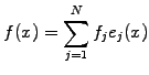
Following the spirit of Hilbert space methods, a function is decomposed on a complete set of nearly orthogonal basis functions $e_j\in\mathcal{B}$

$\displaystyle f(x)=\sum_{j=1}^N f_j e_j(x)$

(1.4.3#eq.1)

These finite-elements (FEM) basis functions span only as far as the neighboring mesh points and need not to be homogeneously distributed. Most common are the normalized ``roof-top'' functions

$\displaystyle e_j(x)=\left\{ \begin{array}{c} (x-x_{j-1})/(x_j-x_{j-1}) \hspace... ...\ (x_{j+1}-x)/(x_{j+1}-x_j) \hspace{5mm} x\in[x_j; x_{j+1}] \end{array} \right.$

(1.4.3#eq.2)

which yield a piecewise linear approximation for

and a piecewise constant derivative $f^\prime(x)$ that is defined almost everywhere in the interval

. Boundary conditions are imposed by modifying the functional space $\mathcal{B}$ , e.g. by taking ``unilateral roofs'' at the boundaries.

**Figure:** Approximation of $\sin(x^2)$ with homogeneous linear finite elements.
$\includegraphics[width=10cm]{figs/AprxFEM.psc}$

Generalizations with ``piecewise constant'' or higher order ``quadratic'' and ``cubic'' FEM are constructed along the same lines. The capability of densifying the mesh where short spatial scales require a higher accuracy is of particular interest. Figure (1.4.3#fig.1) doesn't exploit this, showing instead what happens when the numerical resolution becomes insufficient: around 20 linear or 2 cubic FEM are typically required per wavelength to achieve a precision around 1%. A minimum of 2 is of course necessary to resolve the oscillation.

SYLLABUS Previous: 1.4.2 Sampling on a Up: 1.4 Numerical discretization Next: 1.4.4 Splines