6.2 Cubic-Interpolated Propagation (CIP)

SYLLABUS Previous: 6.1 Splitting advection from Up: 6 LAGRANGIAN METHOD Next: 6.3 Non-Linear equations with

6.2 Cubic-Interpolated Propagation (CIP)

Slide : [ Scheme - Code - Run || VIDEO login]

Introduced a decade ago by Yabe and Aoki [34], a whole family of schemes have been proposed along the same lines, relying on different interpolations to propagate the solution along the characteristics.

Using a cubic-Hermite polynomial, the discretized function and its first derivative $\{x_j, f_j,f_j^\prime\}$ is approximated in a continuous manner with

$\displaystyle \displaystyle F_j(x)=\left[(a_j X -b_j)X + \Delta x f_j^\prime\right]X +f_j\; ; \hspace{7mm}$		$\displaystyle a_j=\Delta x(f_j^\prime+f_{j+1}^\prime) -2(f_{j+1}-f_j)$
$\displaystyle X=\frac{(x-x_j)}{\Delta x}\;\;;\;\; \Delta x =x_j-x_{j-1}\; ; \hspace{7mm}$		$\displaystyle b_j=\Delta x(f_j^\prime+2f_{j+1}^\prime)-3(f_{j+1}-f_j)$

Both $f, f^\prime$ satisfy the master advection equation

$\begin{displaymath}\begin{array}{c}\displaystyle \frac{df}{dt}\equiv \frac{\part... ...\partial x} \right) = \frac{\partial g}{\partial x} \end{array}\end{displaymath}$

(1)

and each is split into an advection (top) and non-advection phase (bottom)

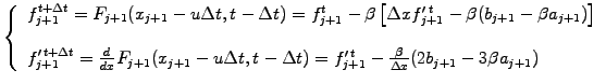
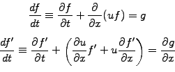
$\displaystyle \left\{ \begin{array}{l} \displaystyle\frac{df}{dt}= 0\\ [5mm] \d... ...rtial g}{\partial x} -\frac{\partial u}{\partial x}f^\prime \end{array} \right.$

(2)

For the advection phase, the solution can be integrated analytically simply by shifting the cubic polynomials $F_j(x,t)=F_j(x-u\Delta t,t-\Delta t)$ along the characteristics

$\displaystyle \displaystyle \left\{ \begin{array}{l} f_{j+1}^{t+\Delta t} = F_{... ...\prime\,t} -\frac{\beta}{\Delta x}(2b_{j+1}-3\beta a_{j+1}) \end{array} \right.$

(3)

without any restriction on the size or the sign of the Courant-Friedrich-Lewy (CFL) number $\beta=u\Delta t/\Delta x$ (exercise 6.01).

For pedagogical reasons, the scheme implemented in JBONE assumes that $\beta\in[0;1]$ so that both quantities $(f_{j+1}^{t+\Delta t}, f_{j+1}^{\prime\, t+\Delta t})$ can be interpolated from only one piece of the piecewise continuous polynomial, namely $F_{j+1}$ defined in the interval $[x_j;x_{j+1}]$ . After an initialization where the function is discretized with cubic-Hermite polynomials by sampling on a grid and the derivative are calculated with centered finite differences, the CIP scheme is implemented as

      double alpha=timeStep*diffusCo/(dx[0]*dx[0]);  //These are only constant
      double beta =timeStep*velocity/(dx[0]);        //  if the problem and the
      int n=f.length-1;                              //  mesh are homogeneous

      for (int j=0; j<n; j++) {
        a=dx[0]*(df[j]+  df[j+1])-2*(f[j+1]-f[j]);
        b=dx[0]*(df[j]+2*df[j+1])-3*(f[j+1]-f[j]);
        fp[j+1]=  f[j+1] -beta*(dx[0]*df[j+1]-beta*(b-beta*a));
       dfp[j+1]= df[j+1] -beta/dx[0]*(2*b-3*beta*a);
      }
      a=dx[0]*(df[n]+  df[0])-2*(f[0]-f[n]);
      b=dx[0]*(df[n]+2*df[0])-3*(f[0]-f[n]);
      fp[0]=  f[0] -beta*(dx[0]*df[0]-beta*(b-beta*a));
      dfp[0]= df[0] -beta/dx[0]*(2*b-3*beta*a);

The applet below illustrates the high quality of this approach, which combines a low level of dispersion with low damping.

**JBONE applet:** press **Start/Stop** to simulate the advection of a box function and to test how cubic Hermite FEM interpolated propagation (CIP) affects the dispersion and the damping of short and long wavelengths superposed in a box function.

Numerical experiments: cubic interpolated propagation

Change the initial condition to Cosine and reduce the spatial resolution down to 4 and 2 mesh points per wavelength to measure how small both the numerical diffusion and dispersion are in comparison with other schemes.
Switch to Cubic--Splines to test an alternative scheme, where cubic splines (1.4.4#eq.1) are used instead of Hermite polynomials to interpolate from any interval in the periodic domain. This allows for arbitrarily large CFL numbers $\vert\beta\vert>1$ as can be tested by choosing TimeStep=21.333 and changing the sign of the Velocity.

Some additional bookkeeping is of course necessary in a code that is intended for $\vert\beta\vert>1$ : exercise 6.01 deals with exactly this problem and can be implemented in a similar manner as illustrated with the Cubic--Spline scheme.

SYLLABUS Previous: 6.1 Splitting advection from Up: 6 LAGRANGIAN METHOD Next: 6.3 Non-Linear equations with